Section 24.1: Introduction to Searching, Sorting, and Big-O
This written lesson just scratches the surface of the content. You will definitely want to watch the videos.
We will be studying 7 algorithms: 2 search algorithms (linear search and binary search) and 5 sorting algorithms (bubble sort, selection sort, insertion sort, merge sort, and quicksort). For each of these 7 algorithms, you must be able to:
understand how the algorithm works. For searching algorithms, you must be able to demonstrate this by listing the items in the array that will be examined in the order in which they will be examined. For sorting algorithms, you must be able to demonstrate this by drawing snapshots of the array after each pass through the array. You'll almost certainly need to watch the videos in order to be able to to do this.
State the big-O running time of the algorithm.
Understand the code for the algorithm.
Computer Scientists use big-O notation to express the efficiency of algorithms in very broad strokes. There are formal mathematical definitions that you will cover in a Discrete Math class. For our purposes, we just need to have an intuitive sense for what the big-O will be for a given algorithm.
To do this, we need to think about a function of "n" (where in is the number of items being processed) that expresses the number of operations that an algorithm would need to perform. The good news is, we don't need to know the exact function. In order to get a good sense of the efficiency of the algorithm, all we need to know is what family of functions the function falls into. Is it a linear function? A quadratic function? A constant function? An exponential function? A logarithmic function? As n gets to be very large, any other considerations, such as constants that might appear in the function, become insignificant.
We write the big-O notation to identify which of these families the function falls into. For example, if it turns out to be a linear function, we write O(n). If it turns out to be quadratic, we write O(n2). If it turns out to be a constant function, we write O(1).
Here's a file with the code for all of the sorting algorithms: sort.cpp
You can view animations of sorting algorithms here.
Section 24.2 Selection Sort
Selection Sort was covered in lesson 9, the lesson on arrays. The idea is that we will find the smallest item in the array and swap it with the first item in the array. We'll keep track of what portion of the array has still not been sorted, so technically I should say "swap it with the first item in that portion of the array that is still not sorted."
The picture below shows snapshots over time of a single array that is being sorted using selection sort. Each line in the picture represents the results after a single pass through the array. The part of the array that is boxed is the part that is sorted. Study the picture to make sure that you could reproduce this on a different set of numbers.
selection sort image
To analyze the efficiency of each algorithm, we are going to be using big-O notation. If you study big-O notation formally it can get pretty complex. We are only going to informally discuss each algorithm to determine which family of functions it falls into. For example, the algorithm might be linear, in which case we would write O(n), pronounced "big-O n". ("n" is the number of items in the array.) The algorithm might be logarithmic, in which case we would write O(logn). Hopefully this will make more sense as we do a few examples.
For selection sort, notice that each row in the picture requires us to look at each element in the array (in order to find the smallest one), so each pass through the array would be O(n). It may actually be a bit more than n or a bit less than n -- technically it's about n / 2 -- but that's not significant for our goal of placing the algorithm in the correct family of functions.
We will be required to perform about n passes through the array. Therefore, the total number of operations will be roughly n2, and we conclude that selection sort is a O(n2) algorithm.
Please refer to the final sorting code file and study the code for implementing selection sort.
Section 24.3 Bubble Sort
bubble sort image
Section 24.4 Insertion Sort
insertion sort image
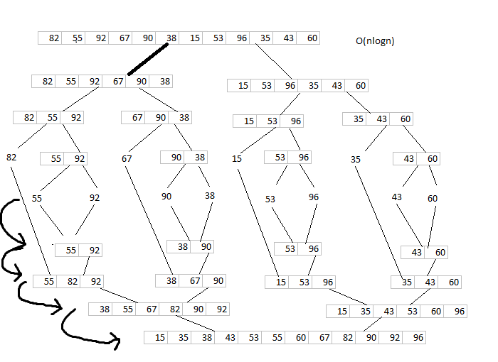
Section 24.5 Merge Sort
merge sort image
Section 24.6 Quicksort
Unlike the other sorting algorithms that we have studied, there are many variations on the quicksort algorithm. In lecture we will be studying one particular approach, which you will be responsible for. The approach in the text is a little different.
The general idea behind quicksort is that we will pick a number, called a "pivot", and we will place all of the numbers less than the pivot on the left side of the pivot, and all of the numbers greater than the pivot on the right side of the pivot. Then we will sort each of those two halves, using the same approach (pick a pivot, place numbers less than the pivot on the left and the numbers greater than the pivot on the right).
There are a number of different strategies that are used for choosing the pivot. Ideally, we could always use the median of all of the numbers as the pivot, but there is no way to calculate that without slowing things down too much. Our strategy will be simple: we will use the last number in the list as the pivot.
You'll also need to know that quicksort is O(nlogn), for the same reasons that merge sort is O(nlogn). And you should take a look at the code in the sort.cpp file.
quicksort image